
PivotTable Features You Need To Know
Many accounting and financial professionals use Excel PivotTables to summarize and report transactional data – sometimes large volumes of transactional data. However, most of these same professionals use only
a handful of the PivotTable features and tools available to create powerful reports in minimal amounts of time. Read on, and in this article, you will learn about some of Excel’s “hidden” PivotTable features. You will be amazed how these features can help you create powerful reports in very little time.
Adding User-Defined Calculations To Your PivotTables
PivotTables offer eleven summarizing calculations, with SUM being the default. However, you can create user-defined calculations in your PivotTables to make them even more suitable to your needs. User-defined calculations in PivotTables take one of two forms – calculated fields and calculated items. Upon creating a calculated field, you treat the results the
same as additional columns of data in your data source. Accordingly, you can click-and-drag a calculated field into your PivotTable the same way as if the field was “native” to the source data feeding into the PivotTable.
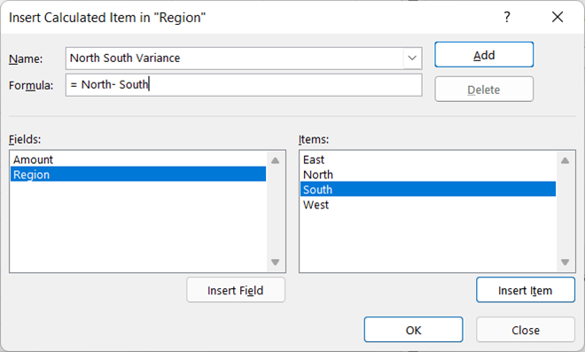
On the other hand, you can create a calculated item from one or more items already in the PivotTable. For example, suppose you have a PivotTable that includes a field named Region. Further, assume the Region field contains four items – North, South, East, and West. Additionally, assume that you want to calculate the variance between the values in the North and South items. In that case, a calculated item would serve you well.
The process for creating these user-defined calculations is relatively easy. First, click on the PivotTable. Next, click the PivotTable Analyze tab of the Ribbon and then click Fields, Items, & Sets, followed by either Calculated Field or Calculated Item. Then, enter your desired formula in the dialog box and click OK to save it. Finally, add the newly-created Calculated Field or Calculated Item to the PivotTable using the traditional PivotTable drag-and-drop process.
Figure 1 illustrates the process of creating a calculated item. Note, however, if you need to create a Calculated Item, you must first click on an item in the PivotTable before starting the process. Of course, if necessary, you can always edit your user-defined calculation by returning to the dialog box where you created the formula.
Creating PivotTables From Data Models
Data models provide a potent option to build PivotTables from multiple ranges of data. However, if you have worked with PivotTables for a while, you already recognize that a PivotTable can have only a single data source. In the past, if you needed to create a PivotTable that incorporates data from multiple ranges, you likely used a VLOOKUP or XLOOKUP-based formula to link data from one range into a second one. Then you built the PivotTable from the range that included the data linked via the formula.
If you opt for data models, using VLOOKUP or XLOOKUP to link data is unnecessary with data models. Instead, if you first convert your data ranges into tables, you can easily create a data model that consists of all the data in all the tables that you include in your data model. And with the data model created, you can easily construct your PivotTable from all the data in the data model.
Perhaps the easiest way of creating a data model is first to ensure that all the data you want to include in the data model resides in tables in Excel. Then, from the Insert tab of the Ribbon, click PivotTable. In the dialog box that appears, check the box labeled Add this data to the Data Model and indicate which columns should be used to relate the tables. Finally, click OK to complete the process. Upon doing so, Excel automatically creates the data model from all the tables in the workbook. With the data model constructed, you can then build your PivotTable using data from any of the tables in the data model.
Setting Default PivotTable Layouts
Unfortunately, many PivotTable users waste substantial amounts of time applying formats to their PivotTables. However, this need not be the case because Excel allows setting default formats for all future PivotTables you create. To establish your default PivotTable layout, click File, Options, Data in Excel. Next, in the dialog box that appears, click Edit Default Layout. Finally, in the Edit Default Layout dialog box, establish the formatting options you want to apply to all future PivotTables you create and click OK. Upon doing so, the options you choose will apply to all future PivotTables you create.
Applying Slicer And Timeline Filters
Slicer and Timeline filters provide easy-to-use, graphical filtering options for your PivotTables. You can apply Slicer filters to any field in a PivotTable. However, as their name implies, you can only use Timeline filters to date-oriented data. To add a Slicer (or Timeline) to a PivotTable, from the PivotTable Analyze tab of the Ribbon, click Insert Slicer (or Insert Timeline). Next, indicate the field(s) you want to filter and click OK. Upon doing so, Excel creates the Slicer (or Timeline) and adds it to the PivotTable. To use the filter, simply click on the items in the filter and the PivotTable filters accordingly.
A bonus associated with Slicers and Timelines is that you can use these filters to modify multiple PivotTables simultaneously. For example, if you have two or more PivotTables created from the same data source, right-click on the Slicer (or Timeline) and choose Report Connections. Then, in the ensuing dialog box, check the box next to each PivotTable’s name to which you want the Slicer (or Timeline) to apply. After doing so, whenever you use the filter, it will impact all the PivotTables selected.
Summary
Many professionals consider PivotTables to be Excel’s most powerful feature. But unfortunately, many of these same professionals remain bogged down and use dated techniques for creating and using PivotTables. Far from an exhaustive list of all the PivotTable features you should use, the four items discussed above can go a long way toward enhancing your PivotTables and reducing the amount of time you spend creating and managing them. So give each of these techniques a try and boost your PivotTable productivity.
You can learn more about PivotTables by participating in K2’s Excel PivotTables For Accountants.