Unpivoting Data with Excel's Power Query Tool
Power Query – a feature available in Excel dating back to 2010 – has emerged as “mainstream” tool for many Excel users. No doubt, Power Query makes it easier for us to access and link data from external data sources, such as our accounting, ERP, practice management, CRM applications. However, one of Power Query’s best features is its ability to “cleanse” and “transform” data to make it more useful and easier to manipulate and analyze. One of the more powerful transformations available in Power Query is its ability to “unpivot” data. In this tip, you will learn how easy it is to take advantage of this feature.
First, the Need to Unpivot
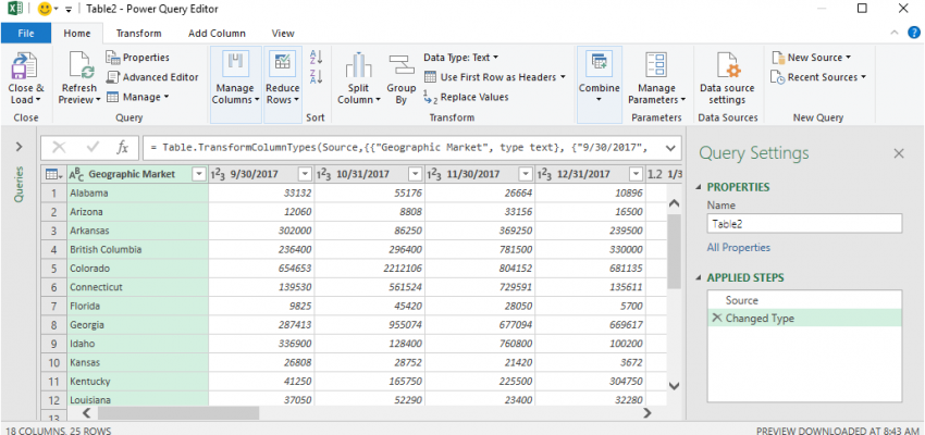
Sometimes when we access data, we find that it has already been summarized in a format that is not particularly useful to us. For example, consider the data pictured in Figure 1 (with several rows and columns hidden for presentation purposes.) Notice that the data is summarized already, with separate columns for each month and rows for each state/province.

While a summarization such as that in Figure 1 might be useful in some cases, in many others it would limit our reporting options. For example, we would find it challenging to create a PivotTable and/or PivotChart with the data already summarized as shown. However, with the “unpivot” feature available in Power Query, we can quickly transform the data to make it more useful and easier to use in other reports, summaries, and analyses.
Accessing Power Query
To begin the process of unpivoting the data, convert the data range to an Excel table, if it is not already in that format. Of course, the quickest way of doing so is to click in the data range and then use a CTRL + T keyboard shortcut. Next, click any cell in the table. Then, if you are running Excel 2016 or newer, click Get Data from the Data tab of the Ribbon to access Power Query. Choose From Other Sources, followed by From Table/Range to load the table into Power Query. At this point, you should see a window that resembles that pictured in Figure 2. Note that if you are running Excel 2013 or Excel 2010, you will need to install the Power Query add-in; upon doing so, you will access Power Query from the Power Query tab of the Ribbon.

If your table has a total column in it, you should delete that column by clicking on it and choosing Remove Columns from the Home tab in Power Query. Likewise, if your table has a total row in it, you should delete that row by choosing Remove Rows from the Home tab in Power Query. Upon clicking Remove Rows, choose Remove Bottom Rows, if your total row occupies the last row of the table. Remember, deleting columns and rows in Power Query does not affect the source data; rather, it only impacts the data as it resides in Power Query. Further, you can “undo” any transformation – such as deleting rows and columns – by simply deleting the transformation from the Applied Steps pane on the right side of the window. Now you’re ready to unpivot your data.
Using Power Query to Unpivot the Data
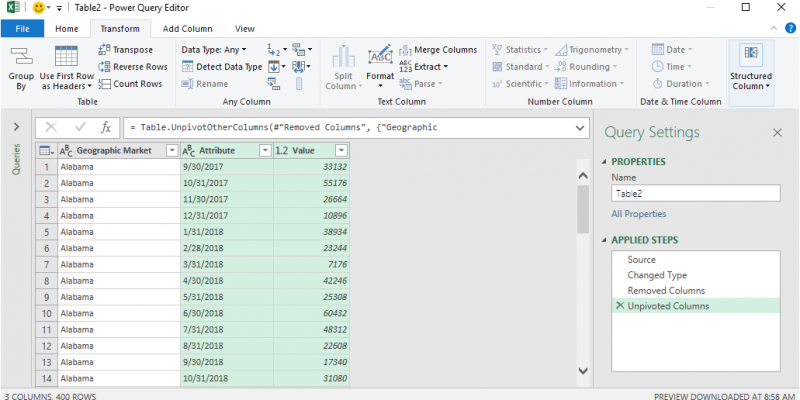
To unpivot the data, select all the numerical columns you wish to unpivot. Generally, you will not select the first column in table. To select multiple adjacent columns, you can simply click on the first one and then hold down your Shift key while you click on the last one. Otherwise, hold down the CTRL key while you click on each column you need to unpivot. With the appropriate columns selected, all that is left to do is to click Unpivot Columns from the Transform tab of the Ribbon in Power Query. Upon doing so, your data will immediately “rotate” into a columnar format such as that pictured in Figure 3.

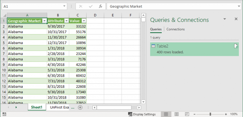
Of course, once you unpivot the data, you can then click Close & Load from the Home tab in Power Query to load the data to a worksheet or to an Excel Data Model. And at this point, you can then use the data in any report, PivotTable, PivotChart, or other environment with no limitations.

Summary
Power Query is becoming a popular tool for Excel enthusiasts for many reasons. One is that it makes it easy for novices to link data into Excel from external data sources. Another is that Power Query provides exceptional data transformation options, and its Unpivot Columns feature is a prime example of these capabilities. So, if you have a need to unpivot your data so that it is more usable in other reports, check out this great feature in Power Query!
You can learn more about Power Query in the following K2 Enterprises seminars:
You can view a video presentation of this tip below.